A brief introduction to data analysis in R
R is a programming language and software, commonly used for statistical computing. What is really cool about it is that it is open source, meaning that all code is openly shared and you don’t need any expensive license to access it. In this brief introduction to R I will go through some of the basic steps you might encounter when pursuing projects in R. This is of course a very (!) brief guide which will mostly be practically oriented. While it is my view that you generally learn programming by doing rather it than reading about it, here are two longer guides that I recommend: An introduction to R and R for data science. It should also be stated that R has a great and helpful community, and most questions you have are probably already answered on stackexchange. Also, ChatGPT is a great coding companion, although it can sometimes trick you into unnecessary complicated solutions…
Content
- Set up
- Core concepts
- Loading a dataset
- Descriptive statistics and visualization
- Basic inference
- Exporting results from R
Basic set up
In order to get started we first have to install R, this can be done here. When installed and opened, it should look like this:
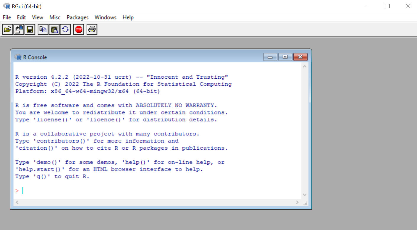
This is the original R Console, and you can use it as it is. For example, you can try simple operations such as 2+2 and you’ll get the output directly. While the R console is basically all you need, working in it is tedious, as you soon will see the RStudio interface makes things much easier. To install RStudio you can go to this site. When you RStudio for the first time it should look something like this:
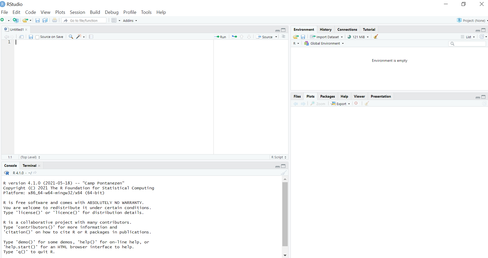
Now you can see that the R Console you saw earlier is in the bottom left box of the interface. Here you can write code directly just as before, try for example once again 2+2. But now we also have three other panels. The top left panel you have your scripts, or code lines, which you can execute from there. For example if you write 2+2, and then mark that line and press Control+Enter, you will see the code being executed in the Console panel below it. The benefit of writing code in the script panel is that you can save the code after you’ve executed it.
Next in the top right corner you have your environment panel, here you can see all your datasets and variables loaded into the session. We’ll come back to this, but just to get a hang of it, try and write A=22 in the script panel, and execute it. What this code does is that it creates a new variable called A, which is assigned the value 22. After you’ve run that code you should see A in the environment panel.
Lastly, in the bottom right panel you have a number of windows available, but the main ones we’ll use are Files, Plots and Help. In the Files window you can see the files of your current R session, in the Plots window you will see your plots and figures, which we’ll come back to. Lastly in the Help window you can see information about different functions. For example try typing help(lm), or help(library), which are some common functions we’ll use.
Creating an R session
Before going any further I want to share one of the most important things I’ve learned about R, which is to have a good data management and project structure. What I used to do when I first started R was to save my datasets and results in different folders, and have my R scripts scattered around the desktop, to do this you click in your script panel and press Control+S, in order to save your R code wherever you like. However, one better way of doing this is to work with R projects. This is a neat way of structuring your R projects and will make everything easier. To do this you press the Files>New Project>New Directory>New Project. When you are here you then name your project to something suitable, for example my_first_project, and you can then click Browse to choose a suitable location for your project, you then click Create Project. Now you’ve created a folder called my_first_project which contains a file called my_first_project.Rproj. Don’t worry about this file for now, all you need to know is that whenever you close your session and want to start up again, all you got to do is to double click this file.
Say that you now want to want to create a new R script, you can press Control+Shift+N to get a new Script window. Try and write 2+2 in it again, and then press Control+S to save it. Now I recommend that you save it within the project folder, and voilá, you are on your way to have a properly structured R session. (One of the benefits of working with projects is that everytime you open the .Rproj file, R will automatically set the working directory to the folder location of that file. While this might not sound important now, this is really convenient later when you download datasets that you want to load into R.)
Data types, data structures and functions
Now that we have our R project up and running, we’ll start to dabble with some key concepts in R. Namely data types, data structures and functions. These are all the core objects in R.
Data types
Previously we learned how to create a new variable called A which contain the value 22. When we do it this way it means that A is treated as a number, and we can for example perform operations with A such as A*2, which returns 44. This is because of how we have created A. If we instead would have created A through A="22", then A would be treated as a line of text or a string, in R we call this data type character. When we do it this way we cannot perform mathematical operations on A, if we would try to take the square root of A through sqrt(A), we would get an error:
> A<-"22"
> sqrt(A)
Error in sqrt(A) : non-numeric argument to mathematical function
See what I did there? I created the variable not through A="22" but through A<-"22", these two are essentially equivalent.
So, how many data types are there? Many, but in my own experience there are three major ones that are good to have an understanding of. The first one is numeric, which is when we store data as numerical values, or numbers. Like A<-22. In reality the numerical class can be both a double or numeric, but it does not really matter for most users. We can test this by assigning A a number and then asking R which class it is:
> A<-2.2
> typeof(A)
[1] "double"
> class(A)
[1] "numeric"
Another class is character, which is when we store data as text or a string.
> A<-"2.2"
> typeof(A)
[1] "character"
> class(A)
[1] "character"
One last important class to be aware of is logical. Logical is a datatype which can take two values, TRUE or FALSE. This datatype emerge when we want to test logical statements operations. To see how it works, see the following examples and play around with it yourself.
> A<-"2.2"
> is.numeric(A)
[1] FALSE
> A <- 2.2
> is.numeric(A)
[1] TRUE
> B <- 5
> A<B
[1] TRUE
> A>B
[1] FALSE
One last thing to note before moving on, is that we can move between datatypes if we need to. For example, say that we have a variable A which contains the number 17 as a character, if we want to change it to a numerical value instead, we can simply use the function as.numeric, if we want to do it the other way around we can use the function as.character(). Here are a few examples on how this works:
> A<-"22"
> B<-22
> A <- as.numeric(A)
> is.numeric(A)
[1] TRUE
> A+B
[1] 44
> B<-as.character(B)
> is.numeric(B)
[1] FALSE
> A+B
Error in A + B : non-numeric argument to binary operator
Similarly we can also move from Logical variables to the character and numeric ones.
> A <- TRUE
> as.numeric(A)
[1] 1
> as.character(A)
[1] "TRUE"
> A<-FALSE
> as.numeric(A)
[1] 0
Data structures
So far we have created objects called A or B, which contain a value of a certain data type. Without going into details these are called vectors of length 1, and can easily be extended to be longer. For example if we want to create a numeric vector of length 2 we can use the c() command.
> A <- c(2,2)
> length(A)
[1] 2
> is.numeric(A)
[1] TRUE
So, a vector is just a collection of values. However, in a vector ALL values need to be of the same data type. Thus a vector has to be either numeric, a character, or logical (or one of the 3 other types I have skipped). We can see how this works by trying to create a vector which contain objects of different data types
> A <- c(TRUE,5)
> A
[1] 1 5
> A <- c("Hello",17)
> A
[1] "Hello" "17"
When we try to contain a logical value and a numeric value in the same vector, both become coerced to numeric values. Similarly when we try to contain a character and a numeric value in the same vector, both become coerced to characters. So, 1 vector 1 data type.
Another data structure closely related to the vectors are matrices. They are simply a vector but with many columns. These also require that all objects are of the same data type, and can be created by the matrix command.
> A <- matrix(c(1,2,3,4),nrow=2,ncol=2,byrow=T)
> A
     [,1] [,2]
[1,]    1    2
[2,]    3    4
Matrices can be useful sometimes, but often we want to store vectors of different data types in the same palce. For example, say that we have a dataset with three columns, such as party, voteshare, in_government. In this case party might be a character vector, voteshare numeric and in_government, could be a logical. In this scenario we want to use dataframes. Dataframes are by far the most common way of structuring data in R. They are just like a matrix, except that each column can be of a different datatype. To create a dataframe we can write:
> example_data <- data.frame(party = c("Party A","Party B"),
+                            voteshare = c(0.43,0.57),
+                            in_government = c(FALSE, TRUE))
> example_data
    party voteshare in_government
1 Party A      0.43         FALSE
2 Party B      0.57          TRUE
> class(example_data)
[1] "data.frame"
In this dataframe we have two rows and three columns, and each column represent a different data type. This is how most datasets are stored and used in R, and another way of formulating it is that each row is an observation, and each column is a different variable, which is measured for each observation.
A good way of sumamrizing the content of dataframes is the str command, which in this case give the following output:
> str(example_data)
'data.frame':	2 obs. of  3 variables:
 $ party        : chr  "Party A" "Party B"
 $ voteshare    : num  0.43 0.57
 $ in_government: logi  FALSE TRUE
As we see, there are two observations, three variables, and each variable are of a different datatype.
Functions and packages
The last thing I’ll talk about before becoming more practical are functions. So far I’ve already used several functions without talking about what they actually are. Going to the basics we can essentially say that functions consist of three things. Input, operations and output.
Take the function we just used, str. The function takes a dataframe as input, then it retrieves all relevant information as an operation, and the output is a summary of the dataframe. Simple as that. Another function we’ve seen is the square root, called by sqrt.
> sqrt(4)
[1] 2
The function takes a number as input, finds the square root as an operation, and gives the answer as output. There are many functions available in R, and it would be impossible to go through all of them. Here is a cheat sheet of some of the most common ones. For example, if we want to create a series of numbers we can write
> 1:10
 [1]  1  2  3  4  5  6  7  8  9 10
this could outputs a vector of numbers going from start_number:end_number.
If we want we can write our own functions. The general syntax for this is
my_function <- function(argument){
   operations
   return(output)
}
For example say that we want to create a function that does the opposite of the square root, it squares the input. Then we can do it like this
square <- function(value){
    output <- value*value
    return(output)
}
If we call this function we then get
> square(2)
[1] 4
> square(4)
[1] 16
There are functions for almost everything, linear regression, correlation, loading datasets, creating plots and more. However, some functions we don’t have access to from the start. For example, say that I want to load an Excel dataset into R (which is the topic of next section), then we either have to write a function that can do this, or we use a function that someone else have written. To do this we can install a package. I like to think of packages as groups of functions that we can load into R. To load an excelfile we can for example load the package openxlsx. We do this by writing
library(openxlsx)
To load a package however, we need to have installed it beforehand. If we try to load a package which is not installed we get an error message like:
> library(lme4)
Error in library(lme4) : there is no package called ‘lme4’
If this is the case we have to install the package, we do this with the install.packages() function.
install.packages("lme4")
Now we can load the package with no problem!
Loading a dataset
Next up, we’ll download a dataset and load it into R as dataframe. Depending on the format of the dataframe there are different commands to use, and different packages we might need. If a file is a .txt or .csv format, the necessary functions are pre-installed R, but if they are in other formats such as .xlsx, we’ll need a package. Some of the functions I often use are summarized in the Table below.
| Datatype | Command | Package |
|---|---|---|
| CSV | read.csv("filename.csv") |
|
| TXT | read.table("filename.txt") |
|
| XLSX | read.xlsx("filename.xlsx") |
openxlsx |
| Stata | read.dta("filename.dta") |
haven |
| SPSS | read_sav("filename.sav") |
haven |
To try these functions download this, this and this dataset and put them in the same folder as your .Rproj file.
If saved correctly, they can then be opened with the following commands
data_csv <- read.csv("cars.csv")
data_txt <- read.table("cars.txt",header=T) #the header=T tells the function that the first row is column names
data_xlsx <- read.xlsx("cars.xlsx",sheetIndex = 1) #sheetIndex tells which "sheet" in the excelfile that should be retrieved
# note that text written after a "#" is seen as a comment in R and will not be executed
Now, lets look at the data. We can do this by clicking the dataframe object in the Environment window, which will trigger the command View(data_csv), if we clicked the data_csv file. We could thus also just write this directly in the command line. As seen all these dataframes are the exact same file, and for now I will just refer to it as data.
One way of summarizing the content of a dataframe is to use the str or summary command. They give the following output.
> str(data)
'data.frame':	50 obs. of  3 variables:
 $ speed: num  16 20 15 10 14 4 24 18 20 13 ...
 $ dist : num  40 56 26 18 60 10 120 42 64 34 ...
 $ model: chr  "tesla" "tesla" "volvo" "volvo" ...
> summary(data)
     speed           dist           model
 Min.   : 4.0   Min.   :  2.00   Length:50
 1st Qu.:12.0   1st Qu.: 26.00   Class :character
 Median :15.0   Median : 36.00   Mode  :character
 Mean   :15.4   Mean   : 42.98
 3rd Qu.:19.0   3rd Qu.: 56.00
 Max.   :25.0   Max.   :120.00
Thus we have two numeric variables and one character variable. However, say that we now only want to use the dist and speed variable, how can we do this? Remember that a dataframe is just a collection of vectors, meaning that dist and speed are just two numeric vectors. If we want to extract them directly we can use the $ symbol, like this:
> data$speed
 [1] 16 20 15 10 14  4 24 18 20 13 11 24  9 19 15 24  7 13 13 20 11 12 14 14 16 23 18 19 20 10 18 20 17 25 13
[36]  8 19 17 24 22 17 12 12  4 10 18 15  7 14 12
Thus when we use the $ dollar symbol we extract the vector of interest. However, say that we want to keep the dataframe format, but only use the two numeric columns, than we can subset the dataframe and overwrite the “old” dataframe in this way.
data <- data[,1:2]
What this code does is that it basically subsets the dataframe such that we only get the first and second column of the dataframe. More generally, if we want to subset a dataframe (or matrix), we can simply select the indexes of interest in the following way data[row_numbers,column_numers], meaning that if we want the first and second column, and only the 10 first observatiosn we can write
> data[1:10,1:2]
   speed dist
1     16   40
2     20   56
3     15   26
4     10   18
5     14   60
6      4   10
7     24  120
8     18   42
9     20   64
10    13   34
Another way of subsetting the dataframe is to write out which variables we want, for example we could write
data["dist"]
Descriptive statistics and visualization
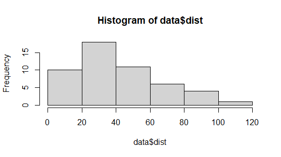
Now that we have our dataframe, how can we analyze it? One way to start would be to visualize it. We can for example plot a histogram for the numeric variables. To do this we can write
hist(data$dist)
then we get a plot in the bottom right panel under the Plots window. It should look like this:
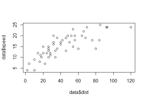
We could also do a scatterplot with the speed and dist variable, using plot like this
plot(data$dist,data$speed)
One popular package often used for visualization is ggplot2. We can install and load the package through
install.package("ggplot2")
library(ggplot2)
Then, say that we want a scatter plot for the dist and speed variable, for each model type alone, we could write the following
ggplot(data,aes(speed,dist))+
  geom_point()+
  facet_wrap(~model)+
  xlab("Distance")+
  ylab("Speed")
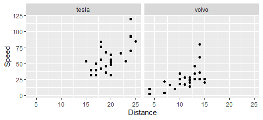
Don’t worry about all the commands for now, you can read more about ggplot2 here, this example is just to show what is possible with the package.
Basic inference
Say that we want to test whether speed and dist are correlated, to do this we could compute the correlation coefficient between the two variables, defined as
$$ r = \frac{\sum_{i=1}^{n} (x_i - \bar{x})(y_i - \bar{y})}{\sqrt{\sum_{i=1}^{n} (x_i - \bar{x})^2 \sum_{i=1}^{n} (y_i - \bar{y})^2}} $$
In R we can compute this using cor like this
> cor(data$speed,data$dist)
[1] 0.8068949
Indeed it seems like the correlation is quite strong. Another way of investigating how these two variables are related is to fit a regression model. To predict speed using dist we can write
model <- lm(speed~dist,data=data)
To see the results we can use the summary function.
> model <- lm(speed~dist,data=data)
> summary(model)

Call:
lm(formula = speed ~ dist, data = data)

Residuals:
    Min      1Q  Median      3Q     Max
-7.5293 -2.1550  0.3615  2.4377  6.4179

Coefficients:
            Estimate Std. Error t value Pr(>|t|)
(Intercept)  8.28391    0.87438   9.474 1.44e-12 ***
dist         0.16557    0.01749   9.464 1.49e-12 ***
---
Signif. codes:  0 ‘***’ 0.001 ‘**’ 0.01 ‘*’ 0.05 ‘.’ 0.1 ‘ ’ 1

Residual standard error: 3.156 on 48 degrees of freedom
Multiple R-squared:  0.6511,	Adjusted R-squared:  0.6438
F-statistic: 89.57 on 1 and 48 DF,  p-value: 1.49e-12
Indeed we find that there is a significant relationship. For every one unit increase in dist the model predicts that the speed will increase with 0.165 steps.
Exporting results from R
The two last things I will discuss is how to export results from R. Figures in R are quite straight forward, after they appear in the Plots window we can export them by clicking the Export button. After this we get a menu where we can write the name and place to store the figure.
Regression tables are a bit trickier. We can see the output directly using the summary function, and could potentially export results from there manually. Another way of doing it is by using a package with functions for this. One I really like is stargazer. To see how it works we install and load it first, and then we can apply it to the regression model we just fit.
stargazer(model,type="text")
With this command we get the regression as a text table which we can copy to a word document for example. There is also the opportunity to get the output as a latex code (for latex documents). Another way is also to output the table as a .html file, which you can then open and copy to your document. This can be done like this
stargazer(model,type="html",out="mytable.html")
With this code you will create a table in the same folder as your .Rproj file, your working directory, which you can then open to access the table, which should look something like this:
| Dependent variable: | |
| speed | |
| dist | 0.166*** |
| (0.017) | |
| Constant | 8.284*** |
| (0.874) | |
| Observations | 50 |
| R2 | 0.651 |
| Adjusted R2 | 0.644 |
| Residual Std. Error | 3.156 (df = 48) |
| F Statistic | 89.567*** (df = 1; 48) |
| Note: | *p<0.1; **p<0.05; ***p<0.01 |
Summary
In this post I’ve tried to discuss how to install R, some of the core concepts of R such as data type, data structure and functions. I’ve then discussed how to load and explore a dataset in R, and how we can apply some simple statistical concepts to the data. Lastly, I’ve discussed how these results can be exported out of R.
